Data

This project will analyse how effective the current channels are in acquiring new customers. Therefore, the following data were collected:

number of newly acquired customers across 118 weeks
the investment in traditional advertising
the number of impressions of Facebook posts initiated by the telecommunications provider
information about media and buzz events, holiday periods, promotions
marketing buzz about the telecommunications provider on Twitter.

The variables and their descriptions are shown below:

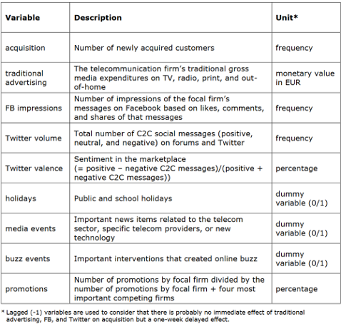
Categorisation

The first approach is to categorise all variables in the form of a market response framework.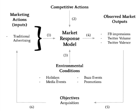

Linear regression analysis

The data has been cleaned prior to its upload into R. Therefore, we can proceed with a linear regression analysis on the data.

All of the variables are numeric.
Since all of the variables have different ranges, the min-max standardisation is used so that each variable’s values are between 0 and 1.

#normalise function
normalize <- function(x) {
  return((x-min(x))/ (max(x)-min(x)))
}

mrm1 = mrm %>% mutate(
  acquisition_n = normalize(acquisition),
  promotions_n = normalize(promotions),
  lag_traditional.advertising_n = normalize(lag_traditional.advertising),
  lag_Twitter_valence_n = normalize(lag_Twitter_valence),
  lag_Twitter_volume_n = normalize(lag_Twitter_volume),
  lag_FB_impressions_n = normalize(lag_FB_impressions)
)

model = lm(acquisition_n ~ buzz.event + media.event + holidays + promotions_n + lag_traditional.advertising_n + lag_Twitter_valence_n + lag_Twitter_volume_n + lag_FB_impressions_n, mrm1)
summary(model)

## 
## Call:
## lm(formula = acquisition_n ~ buzz.event + media.event + holidays + 
##     promotions_n + lag_traditional.advertising_n + lag_Twitter_valence_n + 
##     lag_Twitter_volume_n + lag_FB_impressions_n, data = mrm1)
## 
## Residuals:
##      Min       1Q   Median       3Q      Max 
## -0.32888 -0.10356 -0.01784  0.10310  0.51593 
## 
## Coefficients:
##                                Estimate Std. Error t value Pr(>|t|)    
## (Intercept)                    0.068409   0.054156   1.263 0.209219    
## buzz.event                     0.005015   0.101408   0.049 0.960645    
## media.event                    0.144434   0.041402   3.489 0.000702 ***
## holidays                       0.060637   0.039139   1.549 0.124212    
## promotions_n                   0.275896   0.072476   3.807 0.000233 ***
## lag_traditional.advertising_n  0.296964   0.065331   4.546 1.43e-05 ***
## lag_Twitter_valence_n          0.303281   0.096155   3.154 0.002081 ** 
## lag_Twitter_volume_n          -0.201797   0.070405  -2.866 0.004986 ** 
## lag_FB_impressions_n           0.084160   0.122632   0.686 0.493995    
## ---
## Signif. codes:  0 '***' 0.001 '**' 0.01 '*' 0.05 '.' 0.1 ' ' 1
## 
## Residual standard error: 0.1702 on 109 degrees of freedom
## Multiple R-squared:  0.4277, Adjusted R-squared:  0.3857 
## F-statistic: 10.18 on 8 and 109 DF,  p-value: 1.565e-10

Regression model performance

The performance of the linear regression model will be evaluated in 3 ways:

Model Assumptions
Model fit
Significance of coefficients (via T-tests)

Model Assumptions

Diagnostic plots:

par(mfrow = c(2, 2))
plot(model)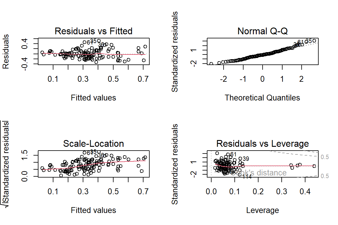

Results:

Linearity of the data: A linear relationship between the predictors and outcome variables can be assumed as the Residuals vs Fitted plot shows no fitted pattern, and the red line is approximately horizontal at zero.
Homoscedasticity: residuals can be assumed to have a constant variance since the residuals in the Scale-Location plot are spread rather equally along the ranges of predictors.
Independence: can be assumed between and within the customers since each customer is a unique individual (ratings by an individual customer are not expected to be dependent on ratings by other customer(s)).
Normality: can be assumed since the normal probability plot of residuals approximately follow a straight line.
Metric scale: all variables are on the metric scale.

Model Fit

The adjusted R-Squared is only 0.3857 meaning that only approximately 38.6% of the variance of the dependent variable is explained by the model ⇒ This suggests that this model is not a good fit.
The p-value associated to the F-statistic is < 0.05 ⇒ this means at least 1 independent variable is significantly related to Acquisition.
The F-statistic of 10.18 is relatively small given the size of our data.
The model has an RSME of 0.314 which is relatively good as there is little variation in the spread of data.

Significance of coefficients (via T-tests)

Before evaluating the significance of coefficients, I did a two-fold cross validation and split the dataset into a training subgroup with 88 observations and a test set with 30 observations.
The two-sample T-test for difference in means was used to validate the partitions as the dataset is entirely numerical.

H0: The means between test and training sets are the same

HA: The means between test and training sets are different

#Two fold cross-validation
split <- round(nrow(mrm1)*0.75)
split

## [1] 88

nrow(mrm1) - split

## [1] 30

set.seed(1)
#Function for two-sample t-test
ttest <- function(training, testing) {
  x1_mean <- mean(testing)
  x2_mean <- mean(training)
  s1 <- sd(testing)
  s2 <- sd(training)
  n1 <- length(testing)
  n2 <- length(training)
  dfs <- min(n1-1, n2-1)
  tdata <- (x1_mean - x2_mean) / sqrt((s1^2/n1)+(s2^2/n2))
  tdata
  pvalue <- 2*pt(abs(tdata), df = dfs, lower.tail = FALSE)
  return(pvalue)
}

trainindex <- createDataPartition(mrm1$acquisition_n, p = .75, 
                                  list = FALSE, 
                                  times = 1)
trainmrm <- mrm1[trainindex,]
testmrm  <- mrm1[-trainindex,]

Derivation of coefficients can be found in the associated .rmd file

Results: Since the p-value of the t-statistic for all explanatory variables are much larger than the 5% significance level, there is not enough evidence to reject the null hypothesis, meaning that the means of explanatory variables in the Training and Test sets are similar.

Dynamic effects

The effort put into marketing sometimes influences sales in future periods. This is known as the carryover effect.
One type of carryover effect is the delayed-response effect. Some of the variables (e.g., traditional advertising and Twitter volume) are delayed by one week. This has been done to account for the delayed effect this action might have on acquisition.
This model takes into account some dynamic effects that are relevant to this case.
However, the inclusion of information from past observations of a series does not necessarily include other omitted variables that may explain some of the historical variations, and that may lead to more accurate forecasts.

Influence of traditional advertising on acquisition

The coefficient for traditional advertising is 0.297 (3sf). This means that traditional advertising and acquiring new customers are positively correlated.
That is, when traditional gross media expenditures increase, the number of newly acquired customers is likely to increase.
Note: 0.297 is a proportional effect.

Influence of FB impressions on acquisition

The coefficient for Facebook impressions is 0.084, which indicates that like traditional advertising, Facebook impressions and acquiring new customers are positively correlated, albeit to a relatively smaller extent.
This means that increasing number of impressions on Facebook will likely lead to increase in the number of newly acquired customers.

Conclusion

Most effective communication channel (traditional advertising, Facebook, Twitter) in stimulating customer acquisition: